Intuition On Database Memory Management
Introduction
I have been working my way through this CMU course which is an introduction to database systems. I’ve primarily been using it as a learning tool for C++ since that seems to be the language of choice for msot implementations of open source database engines.
This week’s project was about implementing a replacer, a buffer pool and a disk interaction mechanism. I thought it was a great way for me to build my intuition on how these things actually work in a database system.
You can find the project here
Memory Representation
So, primarily memory storage for a database is divided into two categories
- Disk memory storage (typically in the form of B+ trees)
- Main memory storage (typically in the form of a hash table)
For this project, the assumption is that the data is stored entirely on disk and then fetched from disk when required.
Here’s what the interaction between the three components looks like.
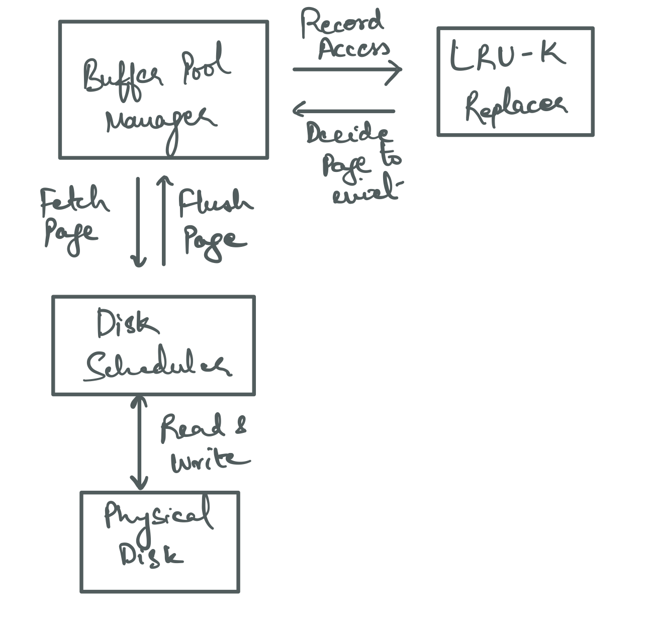
The buffer pool manager is responsible for interaction with the other two components. They never interact with each other directly.
Cache Locality
Before we get into the components, let’s quickly explore cache locality
So, this topic comes up quite frequently when designing database systems and I want to dig into it here. What exactly does cache locality mean?
So there’s typically two classes of storage in a computer - non-volatile and volatile. Non-volatile memory means disk and volatile memory means RAM.
Now, volatile memory can actually be more than just RAM. There’s 3 classes of caches - L1, L2 & L3 - that sit between RAM and the CPU cores. Typically L1 & L2 are faster to access than L3.
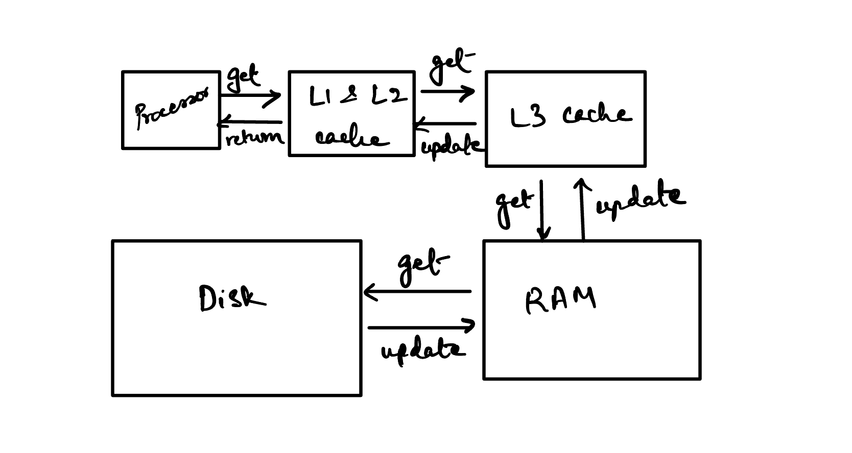
When the CPU needs to access data from “page 2,” a cache miss occurs at the L1 and possibly L2 levels. The hardware then checks the L3 cache, and if another miss occurs, the request is passed to RAM. The buffer pool manager, realizing the page is not in RAM, issues a disk read request via the operating system. The requested page is then loaded into RAM. As the CPU accesses the data from RAM, it gets loaded into the various cache levels (L3, L2, L1) according to the system’s caching policies. Here’s a decent link if you want to read more about this.
Now that we understand how data propagates through these different levels of memory, let’s get into the concept of cache locality. When page 2 is fetched from disk, it’s quite likely that adjacent pages like page 1 and page 3 are also fetched, even if they weren’t explicitly requested. This is due to the principle of spatial locality, where modern systems assume that if one memory location is accessed, nearby memory locations are likely to be accessed soon after. This is often managed by the disk controller or the operating system through mechanisms like read-ahead or prefetching.
So, in scenarios like a sequential scan, the benefit of spatial locality comes into play. Reading page 2 could also bring page 3 and possibly page 4 into faster levels of memory, reducing the likelihood of cache misses and thereby speeding up subsequent reads.
Buffer Pool Manager
Now let’s dive into the actual components.
Think of the buffer pool manager as some memory that has been assigned using malloc when the database engine first starts up. It can hold enough memory for a finite number of pages and the number of pages is sometimes configurable by the end user.
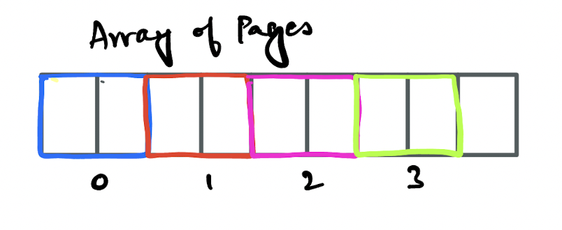
The image above shows a contiguous piece of memory with different colours representing different pages.
Contiguous here is really important and it’s the reason the memory is usually allocated as soon as the database engine starts up versus allocating memory for the buffer pool on a per-need basis.
Having a contiguous piece of memory typically helps with cache locality, which we discussed above.
The numbers in the image above represent the index used to access them when represented in some array like Page[] pages. But don’t assume that the index itself represents the page number, that isn’t the case.
Each of these pages is mapped to a frame which is a concept shared by the buffer pool manager and the replacer. Each of these frames represents one index in the array of pages above.
Now, to determine what page is mapped to what frame, the buffer pool manager makes use of something called a page table. This is just a std::unordered_map<int, int> which tells you which page is stored in what frame.
LRU-K Replacer
Now, we mentioned above that we have finite memory. One of the problems with finite memory is that it is finite. Assume that our buffer pool initially has space for about 10 pages, and our database grows to 25 pages. At some point we are going to want to read data that isn’t in memory and the buffer pool will have to decide which page to evict to make space for the new page.
The logic controlling eviction is called an eviction policy. LRU-K is a variant on the classic LRU replacer algorithm. The only difference with LRU-K is that it takes into account the frequency of access and uses that to decide which frame to kick out.
Notice that I say frame here and not page. This level of indirection is important because the replacer has no concept of the page that is being accessed but the frame that is being accessed. That is, the index in the pages array of the buffer pool manager.
If you want to read more about this, check out the course notes from the lecture on memory management.
It’s a fairly straightforward algorithm and implementing it really helps give you an intuition for what is going on.
Disk Scheduler And Manager
The last piece is probably the most straightforward. This component literally takes read and write requests and reads and writes those pages from or to disk. Nothing significantly complicated going on here.
If you want to follow along with me working my way through the course, you can do so here. And I would highly recommend checking out the course videos, they are a great resource and are freely available on YouTube.